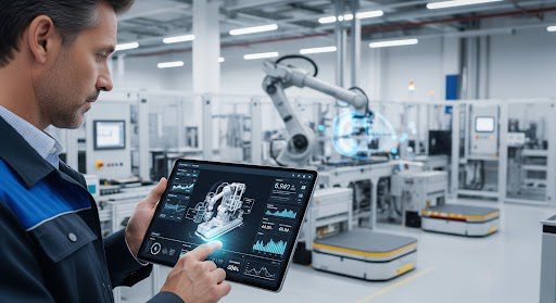
Physical AI
See how a global enterprise SaaS leader rebuilt its SDLC with GenAI in 12 weeks. Accele...
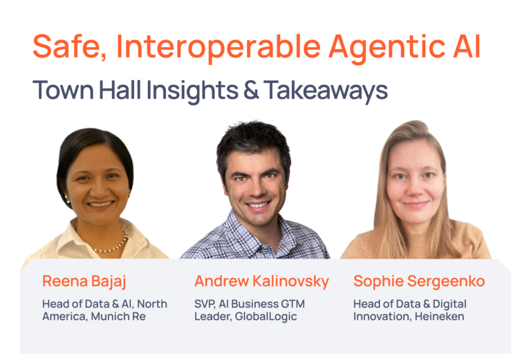
GlobalLogic led the Agentic AI Governance Town Hall for the Gartner CIO and C-Level Com...
GlobalLogic India has been recognized as one of the ET Edge Best Organizations to Work ...
The semiconductor industry is entering a new phase, where value...
Why scaling SDV software needs more than headcount. Inside ...
Learn how AI-powered 5G RAN optimization leverages ...
GlobalLogic shows how Agentic AI transforms workflows into ...
Digital twins are the foundation of modern product ...
As 5G continues its global rollout, the telecommunications ...
As the telecom industry redefines its role, two prominent ...
At GlobalLogic, we’re building systems that don’t just ...
Explore GlobalLogic and AWS webinar on AdTech innovation. ...
Hitachi and GlobalLogic join Google Cloud as Gemini ...
GlobalLogic’s MCP Factory modernizes APIs with Model Context Protocol, enabling...
Digital transformation in the retail industry is not easy. ...
Hi there — how can I assist you today?
Explore our services, industries, career opportunities, and more.